Coordinate Systems

Next: Geometric Description Up: Three Dimensional Element Mechanics Previous: Three Dimensional Element Mechanics

Coordinate Systems

Four different coordinate systems have been used in the development of the curved degenerated shell element. These coordinate systems are defined as follows

1.

The global Cartesian coordinate system which is used as a fixed reference frame for the shell motion, deformation and geometry. The unit vectors ${\bf i}$ , ${\bf j}$ and ${\bf k}$ are in the directions of X, Y and Z, respectively.

2.

The nodal vectors system denoted by ${\bf v}_{1i}$ , ${\bf v}_{2i}$ and ${\bf v}_{3i}$ for node i with its origin at the midsurface. This system is used as a reference frame for the rotations. The nodal vector ${\bf v}_{3i}$ represent the fiber direction which determines the direction on which the fiber inextensibility condition is enforced, and is given by

$\begin{displaymath}{\bf v}_{3i}=\frac{ {\bf x}_i^t-{\bf x}_i^b }{ \Vert {\bf x}_i^t-{\bf x}_i^b \Vert} \end{displaymath}$

(1)

where ${\bf x}_i^t$ and ${\bf x}_i^b$ are the coordinates of node i on the top and bottom shell surfaces, respectively. The other two nodal vectors are picked up such that if ${\bf v}_{3i}$ is close to ${\bf k}$ , then ${\bf v}_{1i}$ and ${\bf v}_{2i}$ are close to ${\bf i}$ and ${\bf j}$ , respectively. Figure (2.1) shows the algorithm used to satisfy this condition.

3.

Natural coordinate system $\xi$ , $\eta$ and $\zeta$ in which $\xi$ and $\eta$ lie in the middle plane, whereas the linear coordinate $\zeta$ spans the thickness direction.

4.

The lamina system denoted by ${\bf x'}$ , ${\bf y'}$ and ${\bf z'}$ is defined at each integration point to describe the directions in which the stresses and strains are obtained. The constitutive relations are written and reduced with respect to this coordinate system. The direction ${\bf z'}$ is the direction in which the zero normal stress condition, $\sigma_{z'}=0$ , is satisfied. As shown in Figure (2.2), the vector ${\bf z'}$ is constructed to be perpendicular to the midsurface at the integration point, while ${\bf x'}$ and ${\bf y'}$ vectors are constructed to be as close as possible from the unit tangent vectors to the $\xi$ and $\eta$ coordinates, ${\bf e}_\xi$ and ${\bf e}_\eta$ , respectively. This is achieved as follows

$\displaystyle {\bf e}_\xi$	=	$\displaystyle \frac{\partial {\bf x}}{\partial \xi} / \Vert\frac{\partial {\bf x}}{\partial \xi}\Vert$	(2)
$\displaystyle {\bf e}_\eta$	=	$\displaystyle \frac{\partial {\bf x}}{\partial \eta}/ \Vert\frac{\partial {\bf x}}{\partial \eta}\Vert$	(3)
$\displaystyle {\bf z'}$	=	$\displaystyle \frac{{\bf e}_\xi \times {\bf e}_\eta} {\Vert{\bf e}_\xi \times {\bf e}_\eta\Vert}$	(4)
$\displaystyle {\bf e}_\alpha$	=	$\displaystyle \frac{\frac{1}{2}[{\bf e}_\xi+ {\bf e}_\eta]}{\Vert\frac{1}{2}[{\bf e}_\xi+{\bf e}_\eta]\Vert}$	(5)
$\displaystyle {\bf e}_\beta$	=	$\displaystyle \frac{{\bf z'} \times {\bf e}_\alpha} {\Vert{\bf z'} \times {\bf e}_\alpha\Vert}$	(6)
$\displaystyle {\bf x'}$	=	$\displaystyle \frac{{\bf e}_\alpha - {\bf e}_\beta}{\sqrt{2}}$	(7)
$\displaystyle {\bf y'}$	=	$\displaystyle \frac{{\bf e}_\alpha + {\bf e}_\beta}{\sqrt{2}}$	(8)

**Figure 2.1:** Nodal Coordinate System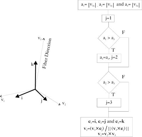

**Figure 2.2:** Lamina Coordinate System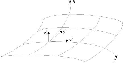

It is worth noting that ${\bf v}_{3i}$ can be obtained as the effective normal vector to the isoparametric shell surface at each node. Alternatively, it could be a given thickness direction, not necessarily orthogonal to the shell middle surface, specified for each node. This latter definition, adopted in this work, is useful for avoiding geometry discontinuities in folded shell situations.

For the purpose of transformation between various coordinate systems, the following two transformation matrices [q] and [s] are constructed from the lamina and nodal vectors, respectively. The matrix [q] transforms from the global system to the lamina system and given as

$\begin{displaymath}{\bf q}=[{\bf x'} \;\; {\bf y'} \;\; {\bf z'}]^T \end{displaymath}$

(9)

while the matrix [s] transforms from the nodal system to the global system and given as

$\begin{displaymath}{\bf s}=[ {\bf v}_{1i} \;\; {\bf v}_{2i} \;\; {\bf v}_{3i}] \end{displaymath}$

(10)

Figure (2.3) shows the relationship between the various coordinate systems.

**Figure 2.3:** The Relationship Between the Coordinate Systems

Next: Geometric Description Up: Three Dimensional Element Mechanics Previous: Three Dimensional Element Mechanics

A. Zeiny
2000-09-06