Variational Principles of the Liquid-Structure Interaction Problem

Next: Modeling of Geometric Nonlinearity Up: The Finite Element Technique Previous: Description of the Finite

Variational Principles of the Liquid-Structure Interaction Problem

The dynamic response of liquids has significant influence on the response of their containers. Inappropriate approximation of the liquid motion may lead to major errors in estimating the seismic response of the container. The liquid pressures and the impact forces form the measurable level of the energy transferred to the tank shell. In addition, the motion of the tank wall is a primary source for the liquid energy. Since this energy transfer occurs simultaneously throughout the liquid boundary, it is essential in the finite element analysis of such problems to use a model that effectively deals with the coupling between the liquid and the tank wall.

The equations of motion of a liquid may be formulated by two different approaches. The Eulerian formulation is obtained by tracking the velocity, pressure and density for all points of the space occupied by the liquid at all instances. The Lagrangian formulation is obtained by considering the history of each particle. In the current investigation, a Lagrangian description of the structure's motion is utilized, which makes it necessary to use a Lagrangian description of the liquid-structure interface in order to enforce compatibility between the structure and the liquid elements. The continuity equation in the Eulerian form is utilized inside the liquid domain to mathematically describe the liquid motion inside the tank.

The liquid in this analysis is considered to be inviscid, irrotational and incompressible. Such simplifying assumptions allow displacements, pressures or velocity potentials to be the variables in the liquid domain. The displacement-based liquid elements may be easy to incorporate in many finite element programs for structural analysis and it may simplify the enforcement of the liquid-structure interface constraints. However, such elements require two or three degrees of freedom per node. In addition, this approach is not well suited for problems with large liquid displacements and requires special care to prevent zero-energy rotational modes. Alternatively, using pressures or velocity potentials as the unknown degrees of freedom requires only one degree of freedom per node inside the liquid domain, which significantly reduces the computational cost of the analysis, yet adequately represents the physical behavior of the liquid. The latter approach is used in this investigation.

Structure Domain

The virtual work statement of the structural domain may be written as

$\displaystyle \delta \Pi_s$	=	$\displaystyle \int_{\Omega_s} \delta \mbox{\boldmath$\epsilon$ }^T {\bf E} \; \... ...d\Omega_s + \int_{\Omega_s}\rho_s \delta {\bf u}^T { \bf\ddot{u} } \; d\Omega_s$
	-	$\displaystyle \int_{\Gamma_w} \delta {\bf u}^T {\bf f}^I \; d\Gamma_w - \int_{\Omega_s} \delta {\bf u}^T {\bf f}^E \; d\Omega_s =0$	(1)

where ${\bf E}$ is the stress-strain matrix, $\epsilon$ is the strain vector, ${\bf u}$ is the displacement vector, $\Omega_s$ is the structural domain, $\Gamma_w$ is the wet surface of the structure, ${\bf f}^I$ is the liquid pressure vector, ${\bf f}^E$ is the body force vector and $\rho_s$ is the mass density of the structure.

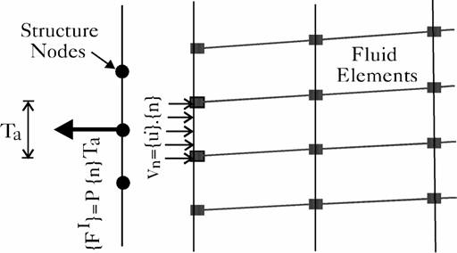
Figure 1: Boundary conditions at a structure node in contact with liquid element

Liquid Domain

Following the work done by Kock and Olson (1991), the variational indicator of an incompressible liquid flowing under gravity field is obtained as

$\begin{displaymath}\Pi_l=\int_{t_1}^{t_2} \int_{\Omega_l} \left\{ \rho_l g y + ... ...triangledown^2 \phi + \rho_l \dot{\phi} \right\} d\Omega_l dt\end{displaymath}$

(2)

or concisely,

$\begin{displaymath}\Pi_l=\int_{t_1}^{t_2} \int_{\Omega_l} P d\Omega_l dt \end{displaymath}$

(3)

where P is the total pressure which may be also written as

$\begin{displaymath}P= P_o-\gamma_l\left[\frac{1}{g} \frac{\partial \phi}{\partia... ...phi. \mbox{{\boldmath$\bigtriangledown$ }} \phi}{2g}+y\right] \end{displaymath}$

(4)

where P_o is the hydrostatic pressure at the point, $\rho_l$ is the mass density of the liquid, y is the Cartesian coordinate measured in a direction opposite to that of the gravitational acceleration g, and $\phi$ is the velocity potential.

Coupled Liquid-Structure System

In order to apply the variational principle to the liquid-structure interaction problem, the liquid and the structure functionals, given by Eq. (1) and (3), are added. The two statements are coupled at the liquid-structure interfaces by

$\displaystyle \dot{u}_n$	=	$\displaystyle \frac{\partial \phi}{\partial {\bf n}}$	(5)
$\displaystyle {\bf f}^I$	=	$\displaystyle P \; {\bf n}$	(6)

where ${ \bf n}=(n_x,n_y,n_z)$ is the outward normal unit vector from the liquid towards the structure. Figure (1) illustrates the interaction between a structure node with a liquid element, where T_a is the tributary area of the structure node.

Next: Modeling of Geometric Nonlinearity Up: The Finite Element Technique Previous: Description of the Finite

A. Zeiny
2000-05-12